Reading Reflection on the Dapper Paper
Introduction
Dapper is Google's distributed tracing system, which laid the foundation for subsequent open‑source implementations such as Zipkin and SkyWalking. Solving the problem of tracing in production environments requires not only a suitable data model but also careful consideration of low code invasiveness and performance impact after deployment, so that the system can be widely adopted and continuously monitored. Dapper's approach is:
- Use span as the basic data structure, modeling a trace as a tree with spans as nodes.
- Modify libraries and use instrumentation to achieve zero code intrusion.
- Employ various sampling techniques to improve performance.
- Build a comprehensive data collection and monitoring infrastructure.
This post explains these aspects in detail.
Data Model
In a microservice architecture, a single user request involves interactions among many services inside the system. Distributed tracing aims to track these interactions, recording the causal order, latency, and other information of all RPCs. Such a call chain typically forms a tree structure, as shown in the figure.
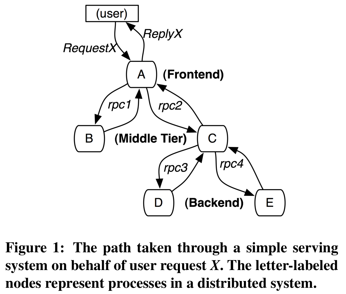
In Dapper, a trace is also a tree structure, where each node is a span. Therefore, the span is the most fundamental data model—it is essentially a log record that describes a single RPC, including the request send time, response receive time, and several ids. Each span has its own id. To represent the tree hierarchy, each span also has a parent id pointing to its parent node. To identify which trace a span belongs to, each span carries a trace id. All spans in the same trace tree share the same trace id.
The two figures below show the information contained in a trace and one of its spans.
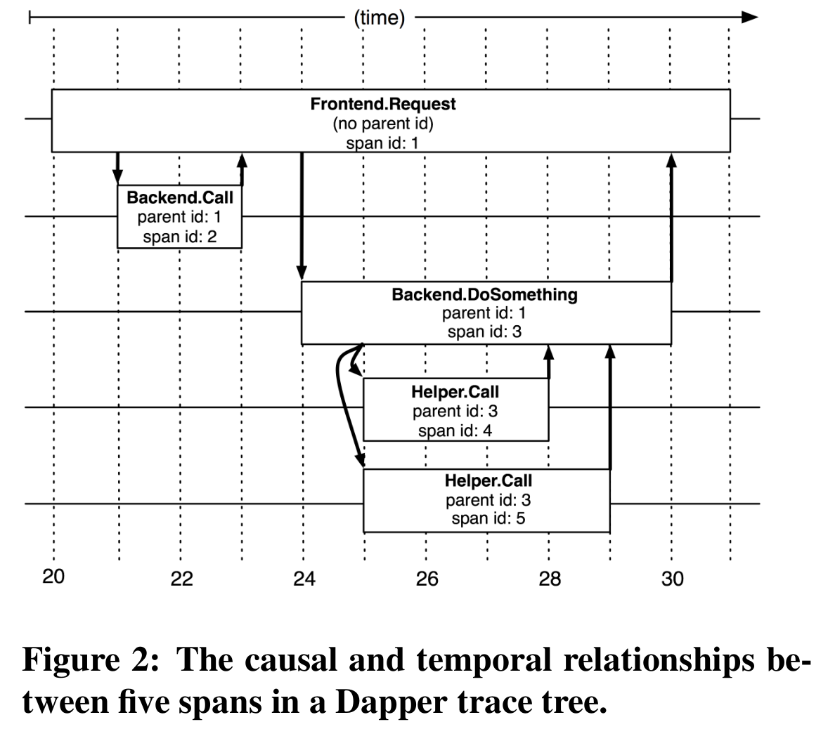
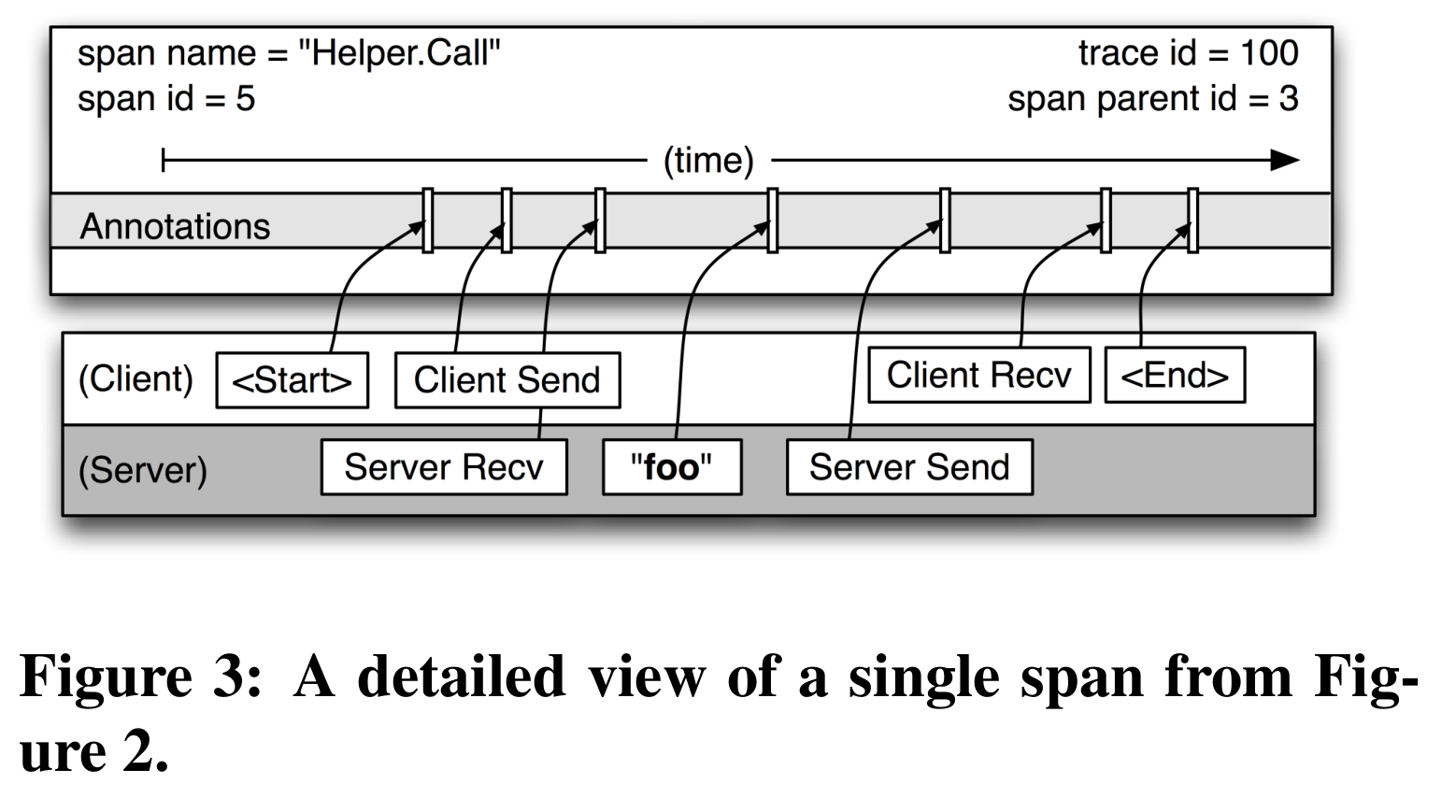
The trace id and span parent id are propagated via RPC attachments. When a node receives a user request, it generates a random trace id and its own span id (this span is the root of the whole trace tree). When this node sends RPC requests to other nodes, it includes these two ids. The node that receives the RPC continues to use the same trace id and uses the incoming span id as the parent id of the span it creates.
Data Collection
The spans on a node are log records generated during its RPC activities. From this perspective, the architecture of Dapper's data collection infrastructure becomes easier to understand. (It is easy to understand from today's viewpoint, but it was not so at the time.)
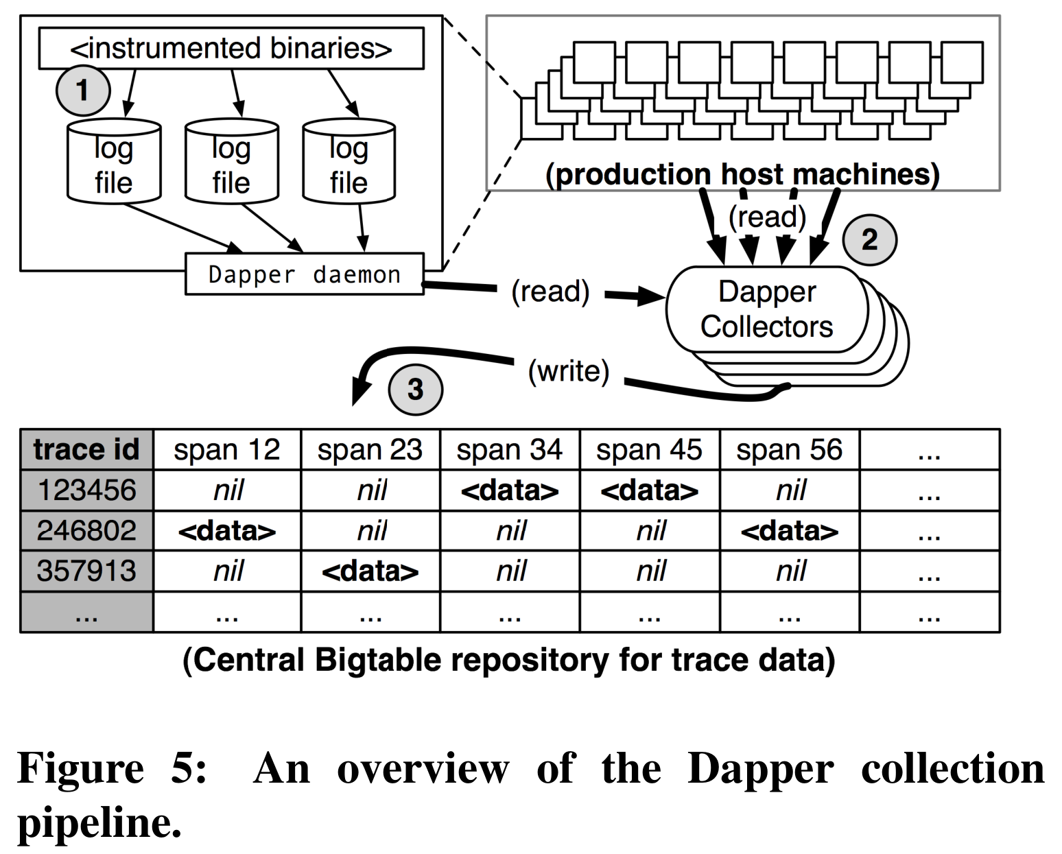
The whole process is relatively simple: applications write span data to local log files; the Dapper daemon (log collection process) reads data from these files and writes them into Bigtable tables. Each row in the table corresponds to a trace, and each column stores a span's data. Bigtable's semi‑structured data model, which does not limit the number of columns, makes it an excellent storage for span data.
The Dapper daemon is deployed in a way similar to a Kubernetes DaemonSet—that is, one instance runs on every machine, responsible for collecting span data produced by all applications running on that machine.
Performance
For tracing to succeed, as many applications as possible must adopt Dapper's mechanism. Otherwise, any unmonitored part would severely affect the visibility of the entire call chain.
Two factors could discourage developers from using Dapper. The first is the need to write extra code. The Dapper team solved this by modifying the widely used RPC libraries and threading libraries inside Google, implementing instrumentation that requires no code changes. Now, applications only need to use the new library versions, which works for both new and existing projects.
The second factor is the performance overhead introduced by tracing, which is hard to compromise for performance‑sensitive applications. The overhead can be split into generation overhead and collection overhead. Generation overhead mainly comes from creating spans and writing span data to disk, both of which increase request latency. The Dapper daemon also competes with other application processes on the same machine for CPU and disk I/O, plus it adds extra network I/O.
Dapper's solution is to sample traces: if only a small fraction of RPCs are traced, the generation overhead has little impact on average latency. The table below confirms this: when the sampling rate is $\frac {1} {1024}$, the average latency barely increases.
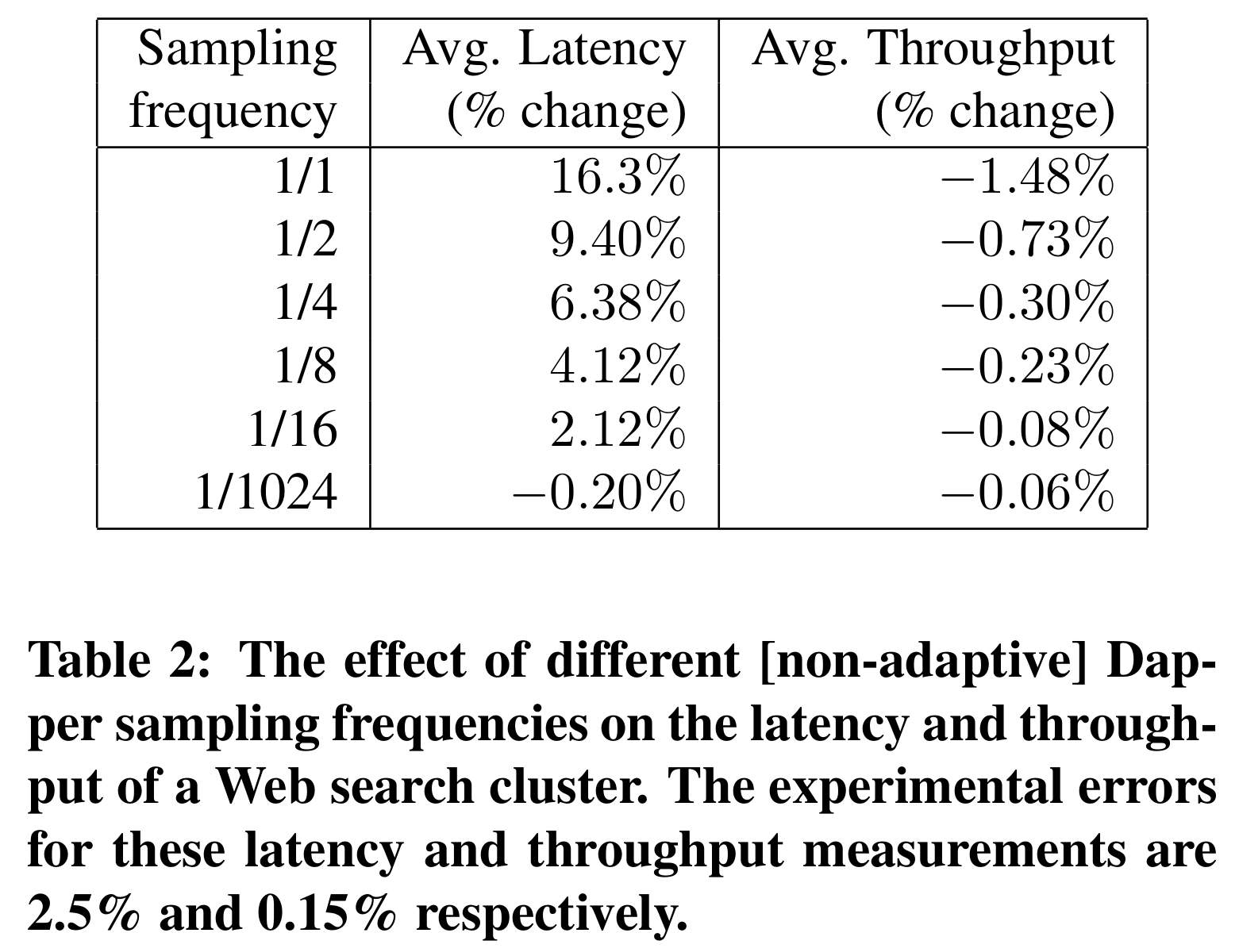
This sampling decision is made at the application level by the node that receives the user request (the root of the trace tree). It decides to trace with probability $\frac {1} {1024}$, generating a trace id accordingly. When other nodes receive RPCs from this node, if the request does not carry a trace id, they will not generate span data.
While this sampling rate seems low, for high‑throughput services it is sufficient to quickly obtain diagnostic information without affecting performance. For low‑throughput services, such a low rate might miss critical data. For those services, increasing the sampling rate is acceptable because it does not create a performance burden. Therefore, Dapper implements adaptive sampling. This feature aims to keep the trace generation rate stable by adjusting the sampling rate based on actual throughput. For example, suppose we want to generate $10$ traces per second. For a service handling $1 \times 10^5$ requests per second, we can set the sampling rate to $1 \times 10^{-4}$; for a service handling $1 \times 10^3$ requests per second, the rate can be $1 \times 10^{-2}$. The rate changes automatically as throughput varies.
With fewer traces generated, the collection overhead naturally decreases. To further ensure that the Dapper daemon does not compete with applications for resources, its priority is set to the lowest level, and it is allowed to use at most 0.3% of a single CPU.
In addition to sampling at the application level, Dapper performs a secondary sampling at the collection daemon. The goal is to control the size of the Dapper table in Bigtable and avoid hitting Bigtable's write throughput limit. This sampling uses a globally configurable parameter $c$ ($c \in [0, 1]$). For each span read by the daemon, a hash function maps its trace id to a value $z$ ($z \in [0, 1]$). If $z \le c$, the span is kept; otherwise it is discarded. Because all spans belonging to the same trace share the same trace id, a trace is either fully collected or completely dropped. This algorithm is clever: it avoids needing a central store to decide which traces to sample, while all collection daemons implicitly agree on the decision.
When I read this section of the paper, I felt that Dapper's secondary sampling principle is very similar to proof‑of‑work in blockchain. In proof‑of‑work, one constantly enumerates the Nonce value in a block to find a value that makes the entire block's hash small enough. Represented in JavaScript code:
2
3
4
5
6
7
8
while (true) {
curBlock.Nonce = rand(); // enumerate a new Nonce value
let z = hash(curBlock);
if (z <= c) {
return "Solved";
}
}Here
cis the threshold for “small enough”, and it adapts to keep the block generation rate constant.
References
- Dapper, a Large-Scale Distributed Systems Tracing Infrastructure
- Bitcoin: A Peer-to-Peer Electronic Cash System
- LLM